Palmer Penguins and regression with a single predictor - SUGGESTED ANSWERS

Application exercise

In this application exercise we will be studying penguins. The data can be found in the palmerpenguins package and we will use tidyverse and tidymodels for data exploration and modeling, respectively.

library(tidyverse)
library(tidymodels)
library(palmerpenguins)

penguins <- na.omit(penguins) # let's get rid of all na values before starting

Please read the following context and take a glimpse at the data set before we get started.

This data set comprising various measurements of three different penguin species, namely Adelie, Gentoo, and Chinstrap. The rigorous study was conducted in the islands of the Palmer Archipelago, Antarctica. These data were collected from 2007 to 2009 by Dr. Kristen Gorman with the Palmer Station Long Term Ecological Research Program, part of the US Long Term Ecological Research Network. The data set is called penguins.

glimpse(penguins)

Rows: 333
Columns: 8
$ species           <fct> Adelie, Adelie, Adelie, Adelie, Adelie, Adelie, Adel…
$ island            <fct> Torgersen, Torgersen, Torgersen, Torgersen, Torgerse…
$ bill_length_mm    <dbl> 39.1, 39.5, 40.3, 36.7, 39.3, 38.9, 39.2, 41.1, 38.6…
$ bill_depth_mm     <dbl> 18.7, 17.4, 18.0, 19.3, 20.6, 17.8, 19.6, 17.6, 21.2…
$ flipper_length_mm <int> 181, 186, 195, 193, 190, 181, 195, 182, 191, 198, 18…
$ body_mass_g       <int> 3750, 3800, 3250, 3450, 3650, 3625, 4675, 3200, 3800…
$ sex               <fct> male, female, female, female, male, female, male, fe…
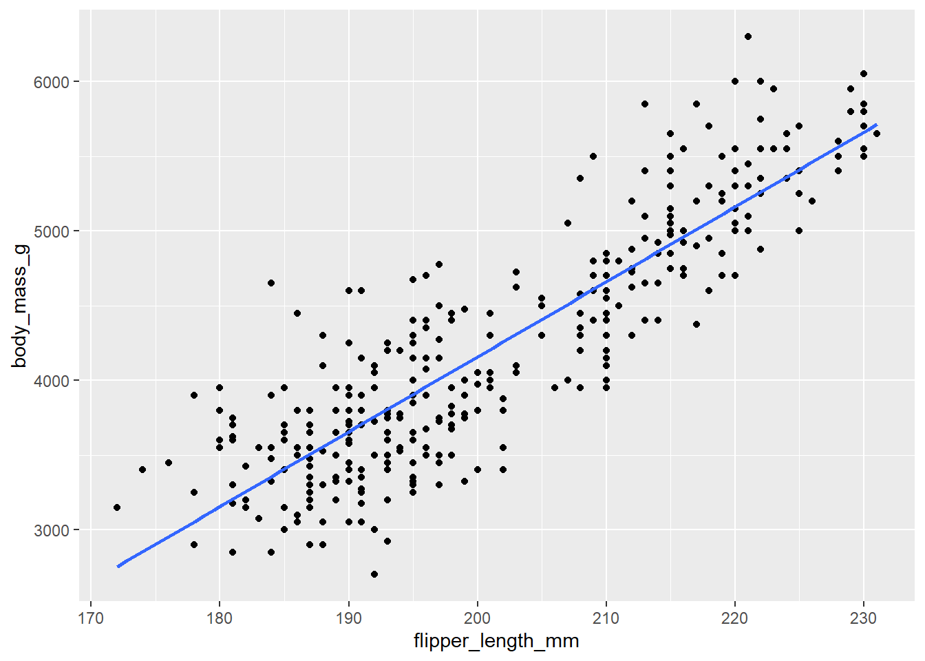
$ year              <int> 2007, 2007, 2007, 2007, 2007, 2007, 2007, 2007, 2007…

Our goal is to understand better how various body measurements and attributes of penguins relate to their body mass. First, we are going to investigate the relationship between a penguins’ flipper lengths and their body masses.

Question: Based on our research focus, which variable is the response variable?

body mass

Demo: Visualize the relationship between flipper length and body mass of penguins.

penguins |>
  ggplot(
    aes(y = body_mass_g, x = flipper_length_mm)
  ) + 
  geom_point() + 
  geom_smooth(method = "lm", se = F)

`geom_smooth()` using formula = 'y ~ x'

Correlation

Your turn (5 minutes):
- What is correlation? What values can correlation take?
Demo: What is the correlation between flipper length and body mass of penguins?

penguins |>
  summarize(r = cor(flipper_length_mm, body_mass_g))

# A tibble: 1 × 1
      r
  <dbl>
1 0.873

Defining, fitting, and summarizing a model

Demo: Write the population model below that explains the relationship between body mass and flipper length. Define each term.

\[ bodymass_i = \beta_o + \beta_1xflipper_i + \epsilon_i \]

Demo: Fit the linear regression model and display the results. Write the estimated model output below.

bm_fl_fit <- linear_reg() |>
  set_engine("lm") |>
  fit(body_mass_g ~ flipper_length_mm, data = penguins)
  
tidy(bm_fl_fit)

# A tibble: 2 × 5
  term              estimate std.error statistic   p.value
  <chr>                <dbl>     <dbl>     <dbl>     <dbl>
1 (Intercept)        -5872.     310.       -18.9 1.18e- 54
2 flipper_length_mm     50.2      1.54      32.6 3.13e-105

\[ \widehat{bodymass} = -5872 + 50.2*flipperlength \]

Your turn: Interpret the slope and the intercept in the context of the data.
- Intercept: When flipper length is 0, we estimate on average a body mass of -5872
- Slopes: For a 1 mm increase in flipper length, we estimate on average an increase of 50.2g in body mass

Another model

Demo: A different researcher wants to look at body weight of penguins based on the island they were recorded on. How are the variables involved in this analysis different?

island is categorical

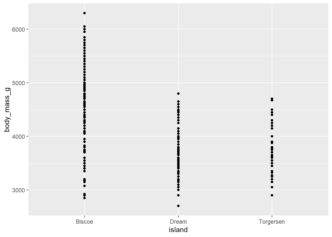
Demo: Make an appropriate visualization to investigate this relationship below. Additionally, calculate the mean body mass by island.

penguins |>
  ggplot(
    aes(y = body_mass_g, x = island)
  ) + 
  geom_point()

penguins |>
  group_by(island) |>
  summarize(mean_bm = mean(body_mass_g))

# A tibble: 3 × 2
  island    mean_bm
  <fct>       <dbl>
1 Biscoe      4719.
2 Dream       3719.
3 Torgersen   3709.

Your turn: Fit the linear regression model and display the results. Write the estimated model output below.

bm_island_fit <- linear_reg() |>
  set_engine("lm") |>
  fit(body_mass_g ~ island, data = penguins)

tidy(bm_island_fit)

# A tibble: 3 × 5
  term            estimate std.error statistic   p.value
  <chr>              <dbl>     <dbl>     <dbl>     <dbl>
1 (Intercept)        4719.      49.4     95.4  2.22e-242
2 islandDream       -1000.      75.4    -13.3  1.74e- 32
3 islandTorgersen   -1011.     105.      -9.67 1.23e- 19

= 4719 - 1000Dream - 1011Torgersen

See next activity for indicator functions!

Demo: Interpret each coefficient in context of the problem.

Intercept: We estimate, on average, the mean body mass of penguins on the biscoe island to be 4719 g.

Dream: We estimate, on average, the mean body mass of penguins on the dream island to be -1000 g less than those on the biscoe island.