Finish Logistic + Intro to Hypothesis Testing
Lecture 20
Duke University
STA 199 - Fall 2023
2023-11-07
Checklist
– Clone ae-20
– Draft Report Due November 15
– Exam-2 released November 16
— Cumulative with a focus on content post Exam-1
Warm Up: What’s a success?
– In practice, we often define a success as the level we are most interested in
– In R, glm defaults to the first level being failure, and the second level being a success
Warm Up: Success
What would R consider a success?
– Variable Smoking: “Smoking” ; “Non-Smoking”
– Variable Smoking: 1 ; 0
Warm Up: Model
\[\log\Big(\frac{p}{1-p}\Big) = -1.9114 - 0.1684 \times exclaim\_mess\]
– What is our response?
– What does p stand for?
Warm Up: Model
\[\log\Big(\frac{p}{1-p}\Big) = -1.9114 - 0.1684 \times exclaim\_mess\]
– Interpret -0.1684 in the context of the problem.
– What is the log odds of a spam email when the email has 3 exclamation points in it?
- What do we do with this?
Log-Odds vs Odds
– The log odds is just the log of an odds ratio.
– An odds ratio is the ratio between the probability of a success and the probability of a failure
\[\frac{p}{1-p}\]
The probability of a spam email given that there are 3 exclaimation points is ~ 0.08. The odds ratio is then:
\[\frac{0.08}{0.92} = 0.087\]
Thus, we can say that the odds of being a spam email are 0.087 times as large as the odds for not being a spam email.
Log-Odds vs Odds
This may make more sense when the odds ratio is > 1. Assume p is the probability that an email is not spam:
\[\frac{0.92}{0.08} = 11.5\] Thus, we can say that the odds of being not a spam email are 11.5 times as large as the odds for being a spam email.
In Summary
– The inverse logit link function and log odds are used to model categorical data, and make our response more symmetric
– We can use the response of log-odds to calculate odds or probabilities
– Can interpret interpret coefficients on the log-odds scale
– Can “math out” (i.e. set X = 3; X = 4) how odds and probabilities change at certain values of X
Statistical Inference
Goals for Today
– Why
– How
of Hypothesis Testing using simulation techniques
Things to consider with hypothesis testing
Null Hypothesis \(H_o\) - “Nothing going on”; “No relationship between variables”
Alternative Hypothesis \(H_a\) - “Our research question”
Things to consider with hypothesis testing
As researchers, we are interested in what’s going on at the population level. We need to make this clear when writing out our hypotheses.
– \(\mu\) - Population Mean
– \(\pi\) - Population Proportion
Example
Suppose we are interested in if the body mass of penguins is larger than 50 pounds.
- That is, we are interested if the true mean body mass of penguins, and hypothesize that their true mean body mass is larger than 50 pounds.
– \(H_o\):
– \(H_a\):
Example
Suppose we are interested in if the body mass of penguins is larger than 50 pounds.
That is, we are interested if the true mean body mass of penguins, and hypothesize that their true mean body mass is larger than 50 pounds.
– \(H_o\): \(\mu\) = 50
– \(H_a\): \(\mu\) > 50
- What if I thought body mass was lower than 50 pounds? What if I thought body mass was different than 50 pounds?
Example
To test this hypothesis, we would need to go out an collect some data. Suppose I collected the body mass of 10 penguins, and found the mean to be 57.4 pounds.
– What is the proper notation for this?
– If you went out to collect data, do you think you would get the sample sample mean?
– Are you comfortable concluding that \(\mu\) > 50 is true based on my data?
Example
Different and No…. because of variability!
Statistical inference is all about capturing variability about a statistic, and using it to make conclusions!
We use this variability to see if any difference we may observe is deemed by “random chance” or not.
ae-20
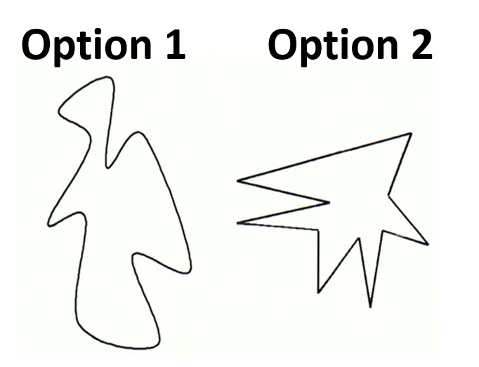
Martian Alphabet
Which letter is Bumba?

Please document your response here
In Summary
– Set up your null and alternative hypothesis at the population level
– Collect data
– Calculate our sample statistic
– Calculate a p-value
– Write a decision
– Write a conclusion
