Logistic Regression
Lecture 18
Duke University
STA 199 - Fall 2023
2023-10-31
Happy Halloween

Super Scary

Checklist
– Clone ae-17
– HW-5 due tonight
– Check Slack for formatting tips
– Schedule Change: Project Draft pushed back to Nov 15th
Feedback for draft will be in Issues tab on GitHub
Must respond to / close Issues specific to your selected data set
Looking Forward
Logistic Regression (Today)
Statistical Inference
– Hypothesis Testing
– Confidence Intervals
Statistical Inference: Hypothesis Testing
Your research question can evolve in 199 a bit as we expand our statistical tool-kit:
– Testing if their are meaningful differences between population parameters (i.e., means or proportions)
Example
Suppose I wanted to test to see if the mean gpa for Duke students was higher than UNC students. We can carry out a hypothesis test to gather evidence if this difference is meaningful or just happens by random chance:
\(H_o: \mu_{duke} =* \mu_{unc}\) \
\(H_a: \mu_{duke} \neq \mu_{unc}\)
Note: You can do something similar with proportions if your response variable is categorical
Statistical Inference: Confidence Intervals
Suppose now instead of testing for a difference, I wanted to estimate what that difference actually is? We can make confidence intervals to estimate a range of plausible values for what \(\mu_1 - \mu_2\) actually is.
Note: You can do something similar with proportions if your response variable is categorical
Tool-Kit
Model Data
– Look at relationships; predictions; estimate probabilities (today)
– Hypothesis Testing
– Confidence Intervals
Warm Up
– What is the difference between R-squared and Adjusted R-squared?
— How are each defined?
— When are each appropriate to use?
Warm Up
– How are each defined?
R-squared: The proportion of variability in our response that is explained by our model
Adjusted-R-squared: Measure of overall model fit
Warm Up
— When are each appropriate to use?
R-squared: when the models have the same number of variables
Adjusted-R-squared: when the models have a different number of variables
Goals
– The What, Why, and How of Logistic Regression
– How to fit these types of models in R
– How to calculate probabilities using these models
What is Logistic Regreesion
Similar to linear regression…. but
Modeling tool when our response is categorical
Start from the beginning
ae-18
What we will do today
– This type of model is called a generalized linear model
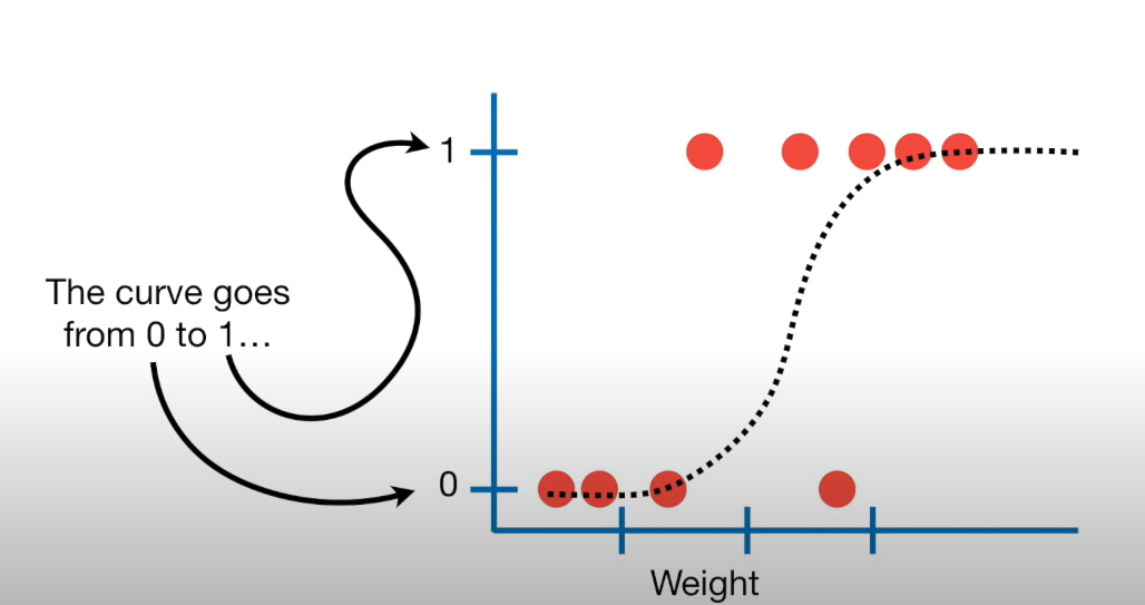
Terms
– Bernoulli Distribution
2 outcomes: Success (p) or Failure (1-p)
\(y_i\) ~ Bern(p)
What we can do is we can use our explanatory variable(s) to model p
Note: We use \(p_i\) for estimated probabilities
2 Steps
– 1: Define a linear model
– 2: Define a link function
A linear model
\(z_i = \beta_o + \beta_1*X_i + ...\)
We use \(z_i\) as a placeholder for our response variable
- But we can’t stop here… we showed that this doesn’t work…
Next steps
– Preform a transformation to our response variable so it has the appropriate range of values
Generalized linear model
– Next, we need a link function that relates the linear model to the parameter of the outcome distribution i.e. transform the linear model to have an appropriate range
– Or…. takes values between negative and positive infinity and map them to probabilities [0,1]
How we start: Logit Link function
– A logit link function takes values between 0 and 1 and maps it to a value between \(-\infty\) and \(\infty\)
The logit link function is defined as follows:
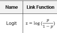
– Note: log is in reference to natural log
What’s this look like
Takes a [0,1] probability and maps it to log odds (-\(\infty\) to \(\infty\).)
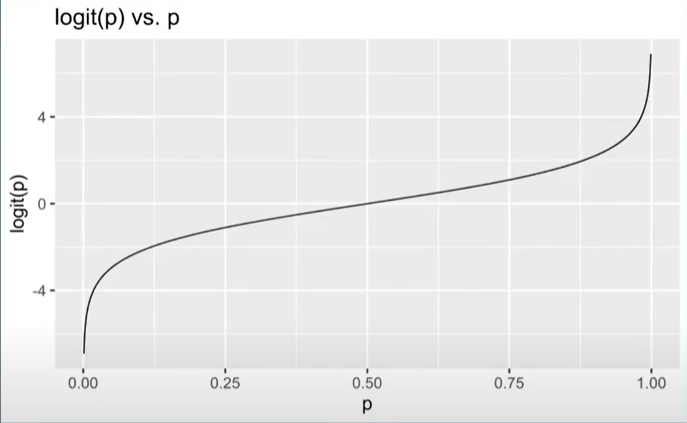
Almost….
This isn’t exactly what we need though…..
Will help us get to our goal
Generalized linear model
– \(logit(p)\) = \(\widehat{\beta_o} +\widehat{\beta}_1X1 + ....\)
– logit(p) is also known as the log-odds
– logit(p) = \(log(\frac{p}{1-p})\)
– \(log(\frac{p}{1-p})\) = \(\widehat{\beta_o} +\widehat{\beta}_1X1 + ....\)
One final fix
– Recall, the goal is to take values between -\(\infty\) and \(\infty\) and map them to probabilities. We need the opposite of the link function… or the inverse
– How do we take the inverse of a natural log?
- Taking the inverse of the logit function will map arbitrary real values back to the range [0, 1]
So
– \(logit(p)\) = \(\widehat{\beta_o} +\widehat{\beta}_1X1 + ....\)
– \[log(\frac{p}{1-p}) = \widehat{\beta_o} +\widehat{\beta}_1X1 + ....\]
– Lets take the inverse of the logit function
– Demo Together
Final Model
\[p = \frac{e^{\widehat{\beta_o} + \widehat{\beta_1}X1 + ...}}{1 + e^{\widehat{\beta_o} + \widehat{\beta_1}X1 + ...}}\]
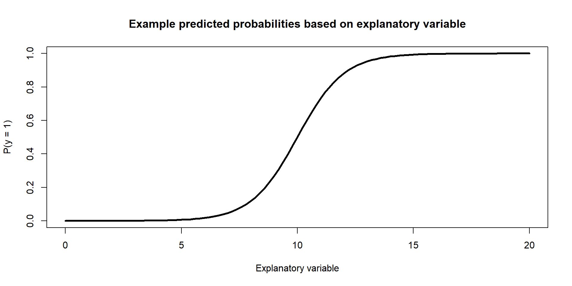
Example Figure:
ae-18
Takeaways
– We can not model these data using the tools we currently have
– We can overcome some of the shortcoming of regression by fitting a generalized linear regression model
– We can model binary data using an inverse logit function to model probabilities of success
